Understanding Bayesian Deep Learning in Binary Classification

Understanding Bayesian Deep Learning in Binary Classification

Let’s explore what is Bayesian Deep Learning (BDL) in the context of binary classification.

Take a look at the interactive version on the Weight & Biases platform.

Introduction to BDL

BDL might sound fancy, but we’re talking about quantify and understanding uncertainty, a crucial factor when you want to manage risks. But, for starting, let’s talk about BDL in a simpler scenario: Classifying cats and dogs.

Uncertainty in Deep Learning

Our approach involves the Monte-Carlo Dropout [2] to work with any pre-trained model. For this tasks of image classification, we picked the EfficientNet (B0 configuration) trained on the ImageNet dataset.

The classifier model features some dropout magic for stochastic output. Here’s a snapshot of what it looks like:

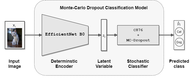
As you can see, the models consist of of two parts. The first part is the feature extractor, which is a convolutional neural network (CNN) that extracts features from the input image. The second part is the classifier, which is a fully connected neural network that classifies the image based on the extracted features.

The feature extractor is a pre-trained EfficientNet model, which is a CNN that has been trained on the ImageNet dataset. This model is deterministic, meaning that it will always produce the same output for a given input. However, the classifier is a stochastic model, meaning that it will produce different outputs for the same input. This is because the classifier uses dropout layers, which randomly drop some of the neurons in the network during training and during inference. This randomness is what makes the classifier stochastic, and allows to measure uncertainty. This is the idea proposed by Gal and Ghahramani [2].

Training the Model with MC-Dropout

We seamlessly integrate the MC-Dropout model into the deep learning workflows. It learns by using classic backpropagation algorithms, with a simple change of the architecture to include dropout layers. The model is trained on the Cats vs. Dogs dataset from TensorFlow Datasets.

The training process is straightforward. These are the results of the training process:

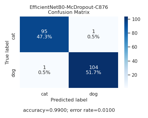
The model is trained with the RMSProp algorithm, with a learning rate of 0.001, preliminary experiments have shown that the SGD and moment base backpropagate algorithms results in underfitting and models with a low generalization.

As you can see, the performance of the model is pretty good, with an accuracy of 99% on the test set. However, the classification is not the important part here. We are interested in measuring uncertainty, what we will do in the next section.

Are You Sure About That?

Predictions aren’t just about saying ‘cat’ or ‘dog’ by selecting the argmax of the model’s output. A MC-Dropout model performs the prediction of the class for a new input differently from a classic model of deep learning. The predictive distribution, i.e., the estimated distribution of classes for a given input, is calculated by sampling the trained model with T stochastic forward passes and average the results:

\[ p(y=C_k|x_i, \mathcal{D}_\text{train}) \approx \frac{1}{T} \sum_{t=1}^T F(x_i, \hat{w}_t) \]

Here, in the right size we have \(F\) as the model, \(x_i\) is the input, \(w_t\) is the sampled weights of the model, approximated by the dropout layers, we sample \(T\) times. And in the left size, \(p(y=C_k|x_i,\mathcal{D}_{\text{train}})\) is the predictive distribution, \(C_k\) is the class \(k\), \(x_i\) is the input, \(y\) is the class of the input, and \(\mathcal{D}_{\text{train}}\) is the training dataset.

Repeating the forward pass can be too slow, that why we implement the 2-step predictive distribution algorithm, a faster computation of the predictive distribution. You can find more details about this algorithm in our paper [3].

The following figures consist of the input image with the true and predicted classes (top left), the predictive distribution and epistemic uncertainty (top right), and a stochastic forward passes distribution by class.

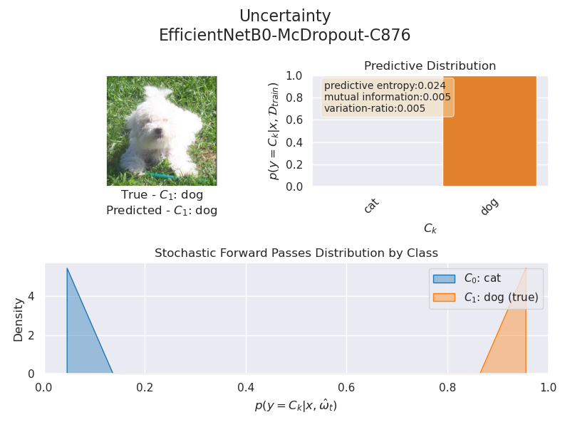
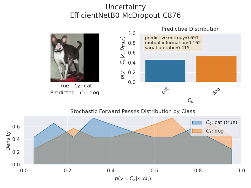
Now, let’s dive into uncertainty. There are two types: epistemic uncertainty (model uncertainty) and aleatoric uncertainty (data uncertainty) [4][5]. Epistemic is like saying, “I’m not sure how the model feels about this”, while aleatoric is more like, “Well, the data is a bit tricky.” In this case, we’re focusing on epistemic uncertainty, which is uncertainty about the model itself.

Uncertainty in Action

The epistemic uncertainty represents the ignorance of the model parameter; it’s also referred to as the model uncertainty because it can be interpreted as the confidence in the prediction. Epistemic uncertainty can reduce this type of uncertainty by adding new samples to our datasets.

They are three measurements of epistemic uncertainty: predictive entropy, mutual information, and variation ratio. For simplicity, we will focus our analysis on predictive entropy, which is calculated as follows:

\[ \mathbb{H}[y|x,\mathcal{D}_\text{train}] = -\sum_k p(y=C_k|x_i,\mathcal{D}_{\text{train}})\log p(y=C_k|x_i,\mathcal{D}_{\text{train}}) \]

The next figure shows some relevant examples from the evaluation set with the higher predictive entropy.

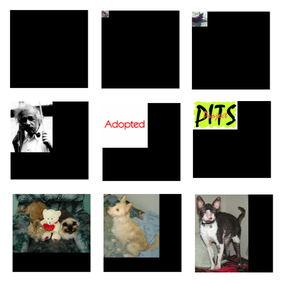
The model has low confidence with these examples, and we can infer that three types of conditions may cause this. The first row shows that an image with a small pixel region containing the a little information is a source of uncertainty. As humans, we also have some difficulty distinguishing these types of pictures due to the image’s low resolution.

The second row contains images out of the distribution of the training set. Pictures of people or text are a real problem, primarily when we can found this type of error in official datasets used by the community.

Finally, the third row contains images of cats and dogs in a weird-looking pose, like the first picture, with a dog looking at the camera that actually is the top of a cat’s head. Or cat and dog with mixed features, like a pointy ear dog and a pitbull fur cat.

When the Uncertainty Matters

Why does uncertainty matter? Because it’s about being in the Real-world scenarios taking decisions with risks. We can’t always be sure about the outcome, but we can be sure about the uncertainty. This is the idea behind BDL, and it’s a powerful tool for managing risks.

Even though the model presented in this article is a binary classifier of cats and dogs, the same principles apply to multi-class classification in the context of medical diagnosis.

We’re applying these lessons in high-stakes situations, like medical diagnosis of HER2 in breast cancer. Check out our work in the her2bdl repository, where we’re bringing BDL to evaluate the expression of HER2 in breast cancer images. For a deep dive into the Her2 Scoring problem with BDL, check the interactive reports or read the paper.

References

• [1] Gal, Y. (2016). Uncertainty in deep learning. University of Cambridge, 1(3), 4.
• [2] Gal, Y., & Ghahramani, Z. (2016, June). Dropout as a Bayesian approximation: Representing model uncertainty in deep learning. In international conference on machine learning (pp. 1050-1059). PMLR.
• [3] Bórquez, S., & Pezoa, R. (2023, August). Uncertainty estimation in the classification of histopathological images with HER2 overexpression using Monte Carlo Dropout, Biomedical Signal Processing and Control, vol 85. DOI: https://doi.org/10.1016/j.bspc.2023.104864
• [4] KENDALL, Alex; GAL, Yarin. What uncertainties do we need in Bayesian deep learning for computer vision?. arXiv preprint arXiv:1703.04977, 2017.
• [5] DER KIUREGHIAN, Armen; DITLEVSEN, Ove. Aleatory or epistemic? Does it matter?. Structural safety, 2009, vol. 31, no 2, p. 105-112.